15 Bad Data Visualization Examples

Data visualization is one of the easiest forms of data representation to understand because our eyes are drawn to colors and patterns. 

For data visualization, charts, graphs, and maps are mostly used. In fact, it is ideal when interpreting big data. However, there are good and bad data visualizations. For a data visualization to be fair, it should follow basic principles.

Most interpreters ignore these principles which lead to bad data visualization, such that it’s difficult and impossible to comprehend. 

Here are some bad data visualization examples.

Bad Data Visualization Examples

1. BBC Avocado Toast Index 

The Avocado Toast Index article by BBC Worklife features some of the bad data visualization examples you’ll find. There are up to 5 of them.

The above data visualization doesn’t tell you anything important. There are up to 5 of them, and the interpreted data was shared between all five graphics. Therefore, to comprehend the data, you must consult all five graphics.

The visualization is about How Many Avocado Toasts Does It Take To Afford A Deposit On A House. Ten cities are used in the study – Mexico City, Johannesburg, Berlin, Tokyo, New York, Sydney, Vancouver, San Francisco, Hong Kong, and London.

Conversely, two cities are used for each graphic. Despite this, it’s difficult to grasp what each of the five graphics is talking about.

The designer represented 100 avocado toasts with one cup and then one dollar notes for an avocado toast price per city. The varying number of avocado toasts consumed and the price of the toasts make the representation disorganized.

The data could be fully prepared and communicated in a straightforward bar chart. 

Check Out: Best Tableau Retail Dashboard Examples

2. Walt Disney’s Companies Worldwide Assets 

Walt Disney has worldwide assets worth billions. If you want to know every company Disney owns, it’s easier to read about it than consulting this infographic by Titlemax. The infographic is a definition of bad data visualization.

This should be highly informative and valuable data visualization if it were not so large and complicated. There is so much information to include, and the designer didn’t do so well with his choice of font size, line weight, circle sizes, etc.

Mickey Mouse’s shape (one of Walt Disney’s most popular characters) is featured, which brings about 3 different circle sizes. Viewers can easily discern that the companies in the larger circle are most important which isn’t so true.

Also, it makes it seem the companies in smaller circles outside the Mickey Mouse frame are less important. Furthermore, the yellow on white color combination is never ideal to use.

Inside the big circles, too many other shapes were used. There are smaller circles, rounded rectangles, sharp cornered squares, and whatnots. Finally, the resolution of such a large data visualization should be at the highest possible rate else reading the small texts will be impossible. 

3. CBSN 

Pie charts are commonly used to show proportions of a whole, but they can easily become misleading when misused.

A notable example comes from CBSN, which created a pie chart showing percentages of Americans who tried marijuana in different years.

Instead of representing a single dataset, the chart combined results from three separate surveys conducted in different years (1969, 1977, and 1985).

This made it look like the percentages were cumulative or simultaneous, leading viewers to believe that the data was interconnected when it wasn’t.

The slices of the pie chart also failed to add up to 100%, violating one of the fundamental principles of pie charts. A better approach would have been to use a bar chart with clear labels for each year to avoid confusion.

4. The Economist, Why ticket prices on long-haul flights have plummeted

The Economist isn’t a publication you would expect a bad data visualization example from but here’s one. The core here is the featured protractor. 

You would expect to grasp a relationship between long-haul flights and their ticket prices. However, what you get are overlapping lines such that differentiation is a problem. 

The protractor features two lines. The blue-colored lines are for transatlantic flights while the ash-colored lines are for other flights. There are three axes with two being Distance in Km and the other, Change in price of economy-class tickets.

Since the length of the lines depends on the flight’s distance, some lines are terse. Hence, it’s difficult to trace them to grasp the percentage change in ticket prices. Furthermore, the actual prices of the flight tickets are not pointed out. 

Except for their not-so-straightforward titles, the three graphs featured below the page are easier to understand. The first represents shares of Norwegian seats on six transatlantic routes, and the second represents jet fuel $ per liter. In comparison, the third represents average ticket prices on six transatlantic routes. 

5. Venezuelan elections

Cylindrical bars are another example where design choices distort reality by exaggerating differences between values.

In Venezuelan election results visualization, cylindrical bars were used to represent vote percentages between two candidates—one receiving 50% and another receiving 48%.

Despite only a 2% difference in votes, the cylindrical bar representing 50% was disproportionately larger than its counterpart, creating the illusion that one candidate was far more popular than the other.

Such visualizations deliberately mislead viewers by exploiting design elements rather than presenting accurate proportions.

6. Cherry-picking

Cherry-picking involves selectively presenting data points that support a narrative while ignoring broader trends that might contradict it.

For instance, pharmaceutical companies have been criticized for presenting clinical trial results that highlight positive outcomes while omitting adverse effects or inconclusive findings.

Another example comes from climate change graphs that show temperature stability over short periods while ignoring long-term warming trends.

Cherry-picking distorts reality and undermines trust in the data being presented. Ethical data visualization requires transparency and inclusion of all relevant data points.

7. ASEC Data, Household Income Percentiles 

This was supposed to be a simple double bar graph, but the designer got the opposite in trying to make it simple.

The graph was meant to represent household income percentiles for 2017 and 2018. However, it was labeled 2017 and 2016. This alone renders this chart unreliable since you cannot grasp what the data is representing.

If you want to utilize this graph, you’ll have to consult the original ASEC data to verify the variables. Nevertheless, with 2017 coming before 2016, 2016 could be an error.

As a double bar graph, the household income percentiles are represented side by side. While the yellow and light blue color combination isn’t awful, a stronger color variation would be better. For example, yellow and standard blue color.

The next thing wrong with this data visualization is the alignment of the text within the bars. You would need to twist your head or rotate the image on your device to read it which can be uncomfortable.

Furthermore, with the dollar cutoff figures at the y-axis, there’s less need to write the actual figures within the bars.

8. Vox, All life on Earth, in one staggering chart

The first thing you’ll notice from this Vox data visualization is its length. That’s the first reason why the visualization is bad. The graph won’t easily fit on any web page, so it’ll take a viewer multiple scrolls to view all the details.

The graph shows all life on earth which includes all plants, animals, and humans. With plants at 450 Gt C, Animals at 2 Gt C, and Humans at 0.06 Gt C.

Looking at the graph, there are more plants than both animals and humans. Also, there are more animals than humans.

It’s the simple fact the chart aimed to interpret, but the choice to use 3 dimensions was a flaw that made it complicated. Most viewers who look at this data visualization will perceive more to it than the fact mentioned.

It would be difficult to represent the actual figures of plants, animals, and humans in the world – or even their size ratio – in a graph. This makes the lengthiness more irrelevant.

9. Bloomberg, Polluted Cities 

If you’re a regular Bloomberg reader, you’ll know this is the standard way the publication prepares their bar graphs. They aren’t totally bad, but they aren’t the best either.

In this particular graph, Bloomberg is not just representing polluted cities in India and China. The percentage increase in these cities from 1998 to 2016 is also being represented.

There are 20 cities in total with 10 Chinese cities and 11 Indian cities. Both are differentiated with ash and white colors, respectively.

The first thing wrong about his chart is how the labels are placed – far away from the graph. Although this is due to the inclusion of the -% and all but one city has a positive increase in pollution, it links the bars somewhat abstruse.

The designer employs a progressive pattern in arranging the cities. However, there are no start and endpoints. Also, you can’t point out just how much of a percentage increase in population was recorded for each year. 

Finally, the use of an all-black background is always not ideal when preparing a data visualization.

10. Visual Capitalist, 80 Trillion World Economy One Chart 

In an article on the 80 Trillion World Economy One Chart, Visual Capitalist features this data visualization prepared by Howmuch.net. The graphic represents the revenue and percentage of the economy of all countries.

Looking at the visualization, you can only easily pick out countries with booming economies which include the United States, China, Japan, Germany, France, etc. If your country doesn’t have a major economy, it’s difficult to find it.

Another thing wrong with the chart is positioning. It’s represented in a circle which can be associated with the Earth’s spherical shape. However, the countries are placed just anywhere which doesn’t mean anything.

Nevertheless, countries of the same continent are positioned close to each other but the sizes are not relative.

The positioning makes it hard to sum up all the revenue of each economy and percentage to check if it equals 80 Trillion and 100 percent respectively. 

Furthermore, the shapes representing the countries are unusual. Although the size of a country’s economy determines its size, nothing relates the shape’s size to the size of the full circle. 

11. P&G Annual Report 

Here we have a data visualization of the P & G annual report. The visualization represents sales by business segment, geographical region, and market maturity in the year 2018. It also displays financial highlights for five previous years (2014 to 2018).

Thanks to the alignment and orderliness, this visualization could easily pass for a properly prepared one. However, there are a few errors.

First of all, the light blue background color doesn’t sit well with white texts. Furthermore, similar colors are used in the charts such that it could be difficult to pinpoint the chart. Thankfully, the yellow color makes it more noticeable.

Donut charts are not the best when it comes to representing more than four categories. In such charts, the categories are separated by areas and lengths, making them difficult to distinguish. This is why it’s easier to grasp the last chart and the first two charts.

Furthermore, the visualization features a legend at the top which is somewhat distant from the charts. Hence, there’s a need for constant head movement, which can inconvenience a viewer. 

12. World Debt in One Visualization 

How much do world governments owe? As of 2018, the figure was estimated at $63 trillion as represented in this data visualization. Visual Capitalist prepared the chart.

The United Nations Of Dept graphic by Visual Capitalist is grotesque and it has a lot to do with the shapes used. Varying shapes – with some very bizarre ones – were featured.

To properly represent data visually, it’s ideal to stick with regular shapes to make it intuitive. Furthermore, they are easier if you want to calculate areas for sizes.

Like the 80 Trillion World Economy One Chart mentioned earlier (still from Visual Capitalist), it is difficult to locate countries with small debts. Only countries like the United States, Japan, China, Italy, etc., with large debts, are easily located.

The color scheme of this data visualization doesn’t sit right either. A lot of similar colors were used to represent most countries in which very abstract colors were used in one or two places.

Finally, this visualization holds no value logically. This is because countries and companies owe each other. Should each country’s liabilities be crossed with their assets, there’ll be zero debt.  

13. Treemaps 

Treemaps are designed to represent hierarchical data using nested rectangles sized according to value, but they can easily become illegible when overloaded with information.

This example involved a treemap attempting to classify countries by population and continent simultaneously.

The visualization crammed too many categories into small spaces without clear labels or logical organization, making it difficult for viewers to extract meaningful insights.

Overcrowded treemaps fail because they prioritize quantity over clarity. Simplifying the design by focusing on fewer categories or using alternative formats like bar charts can make such visualizations more effective.

14. 3d Chart Example

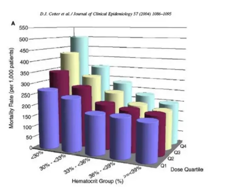
Adding unnecessary 3D effects to charts often makes them harder to read and interpret accurately.

This is a well-known example is a 3D pie chart used by a corporate presentation that distorted angles and areas so much that viewers couldn’t gauge proportions correctly.

The 3D perspective skewed the sizes of slices based on their position in the chart rather than their actual values. While visually striking, such designs sacrifice clarity for aesthetics and fail to communicate data effectively.

Flat designs are far superior because they allow viewers to focus on the data itself without being distracted by visual distortions.

15. Misleading Scales

Using inconsistent or distorted scales can completely misrepresent trends in data visualization. This is a famous example that comes from a graph depicting electricity price changes in Spain over time.

After 2012, the horizontal scale was altered from yearly intervals to quarterly intervals without any explanation. This change created the illusion of reduced price increases under specific policies when prices were actually rising steadily over time.

Misleading scales manipulate viewers’ perceptions and distort reality, often for political or marketing purposes. Consistent scaling is essential for accurate representation.

Bottom Line 

Bad data visualizations can mislead audiences and hinder effective communication of insights.

From truncated axes to overcrowded designs, these examples highlight common pitfalls that should be avoided at all costs.

By prioritizing clarity, accuracy, and thoughtful design principles, we can ensure our visualizations effectively convey their intended messages.

Enjoyed the post?

Share on Pinterest